EDIT (10/12/2020): Updated code to properly label y-axis as PC2.
Recently a friend of mine asked if I had any experience importing an skbio.stats.ordination object in R. I hadn’t, unfortunately, as I usually work with QIIME2 & Python in tandem. I do expect that I’ll be using R more often as my PhD progresses so I decided to take a stab at a very simple way to extract and plot the data from this format.
When you export an skbio ordination object, the text file contains entries for the eigenvalues, proportion explained, and sites (analogous to samples in what I do). Additionally, if the ordination is a biplot, it will contain entries for species as well (analogous to microbes in what I do). There are also spaces for “Biplot” and “Site constraints” which I’m not familiar with. These entries are basically stored in sub-TSVs so this snippet just takes each of these set of values and extracts them to their own data frame. Then I wrote some rudimentary code to plot the samples as points and features as arrows. Of course, this can be snazzed up with fancy ggplot2 accoutrements but for this demonstration I kept it relatively simple.
library(ggplot2)
get_ord_dataframe <- function(lines, linestart){
header_line <- strsplit(lines[linestart], split="\t")[[1]]
num_rows = as.numeric(header_line[2])
num_cols = as.numeric(header_line[3])
if (num_rows == 0){return(data.frame())}
data <- strsplit(
lines[(linestart+1):(linestart+num_rows)],
split="\t"
)
names <- unlist(lapply(data, function(x) x[1]))
coords <- lapply(
data,
function(x) strsplit(x[2:(2+num_cols-1)], split="\t")
)
coords <- data.frame(
matrix(
unlist(coords),
nrow=length(coords),
byrow=T
),
stringsAsFactors=FALSE
)
coords[] <- lapply(coords, as.numeric) #make numeric
rownames(coords) <- names
return(coords)
}
lines <- readLines("results/tutorial/data/ordination.txt")
# format is as follows Eigvals, Proportion explained,
# Species, Site, Biplot, Site constraints
eigvals <- as.numeric(strsplit(lines[2], split="\t")[[1]])
num_axes <- length(eigvals)
prop_explained <- as.numeric(strsplit(lines[5], split="\t")[[1]])
species_linestart = min(grep("^Species", lines))
species_coords <- get_ord_dataframe(lines, species_linestart)
norm_vec <- function(x) sqrt(sum(as.numeric(x)^2))
species_coords$magnitude <- apply(species_coords, 1, norm_vec)
species_coords <- species_coords[order(-species_coords$magnitude),]
sites_linestart = min(grep("^Site", lines))
sites_coords <- get_ord_dataframe(lines, sites_linestart)
biplot_linestart = min(grep("^Biplot", lines))
biplot_coords <- get_ord_dataframe(lines, biplot_linestart)
constraints_linestart = min(grep("^Site constraints", lines))
constraints_coords <- get_ord_dataframe(lines, constraints_linestart)
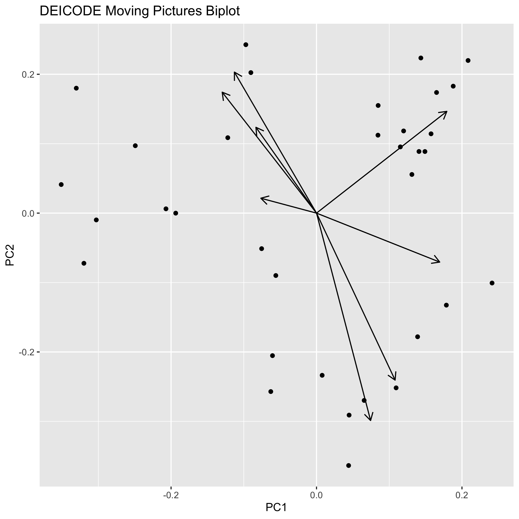
ggplot(sites_coords, aes(x = X1, y = X2)) +
geom_point() +
geom_segment(
data=species_coords[1:8,],
aes(x=0, y=0, xend=X1, yend=X2),
arrow = arrow(length=unit(0.3, "cm"))
) +
xlab("PC1") +
ylab("PC2") +
ggtitle("DEICODE Moving Pictures Biplot")
ggsave("deicode_mp_biplot.png")