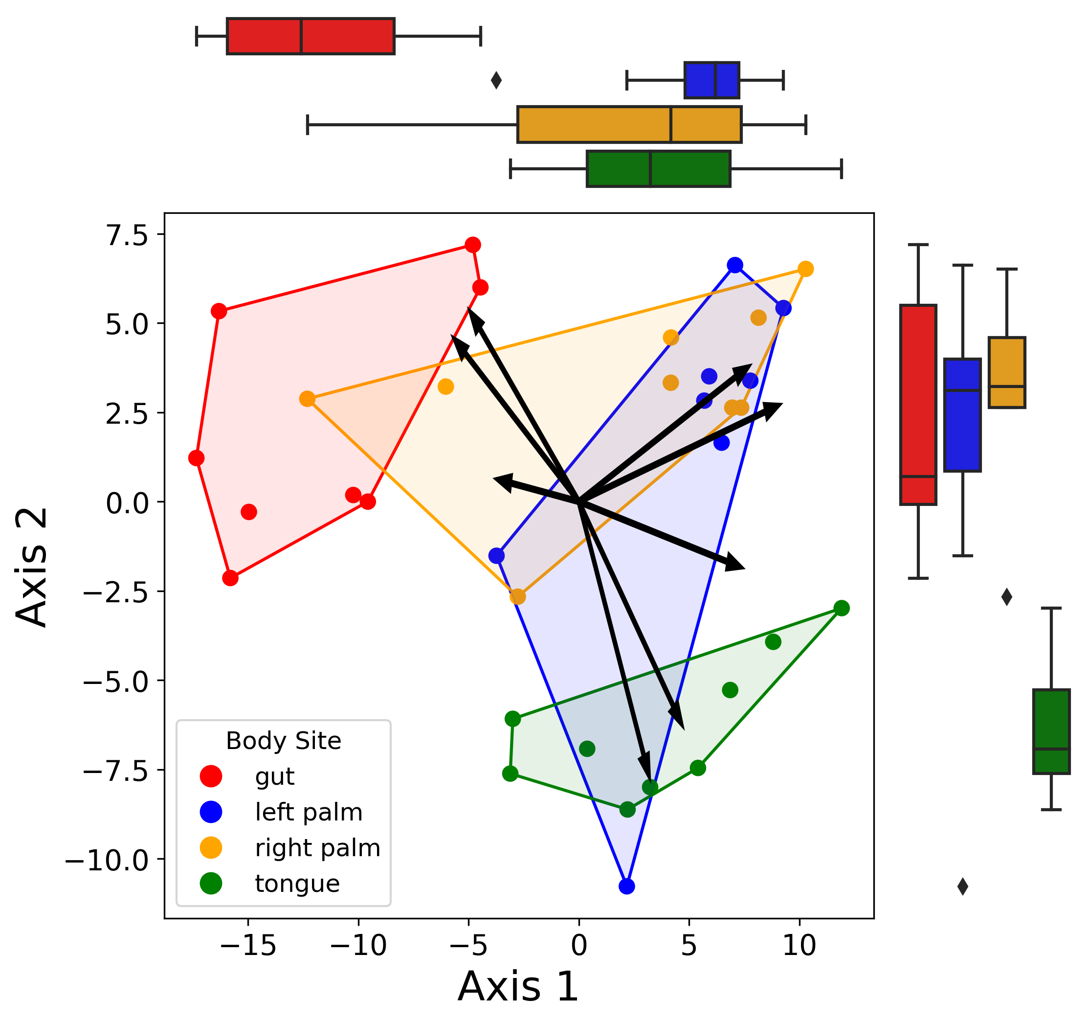
I recently came across a really nice visualization of a biplot wherein the different groups were summarized by a convex hull and the x and y axes had marginal boxplots colored by the same groups.
This plot was made in R through ggpubr but I wanted to see if I could recreate it in matplotlib as I am more familiar with it.
The key aspect here was learning how to compute and plot a convex hull in Python (turns out to be easier than I had anticipated).
This snippet will be similar to my previous post about plotting a biplot in matplotlib.
For those unfamiliar, a convex hull of a set of points is basically the smallest possible convex shape that includes all the points. Think about a rubber band stretched taut around a point cloud - there are no “dips” or other aberrations that would cause the shape to instead be referred to as “concave”. In Python, we can represent a convex hull as the set of ordered vertices comprising this shape. By connecting these ordered points with line segments, we can visualize the 2D variance of the set of points of interest.
In Python, I found that the easiest way to compute this set is with SciPy.
SciPy has a nifty implementation in the spatial module to easily generate a convex hull of a given set of points.
A ConvexHull object has two primary attributes of interest: simplices and vertices.
simplices represents the indices of the points of the hull facets while vertices are the indices of the hull vertices in counterclockwise order (for 2D).
I prefer to use vertices but it should be noted that the default return value does not “connect” the last point to the first point so this must be done manually.
See the documentation here.
The marginal boxplots are fairly straightfoward - I used matplotlib’s GridSpec functionality to create a 2 x 2 subplot with one big axis for the biplot and 2 smaller axes on the top and right of the large one. Overall, I think this type of plot is great for quickly visualizing the differences in groups on both axes.
from matplotlib.gridspec import GridSpec
from matplotlib.lines import Line2D
import matplotlib.pyplot as plt
import numpy as np
import pandas as pd
from qiime2 import Artifact
import scipy
import seaborn as sns
from skbio.stats.ordination import OrdinationResults


metadata = pd.read_csv("data/sample-metadata.tsv", sep="\t",
                       index_col=0)
ord_results = Artifact.load("data/ordination.qza").view(OrdinationResults)

def reconstruct_comp(
    ord_results: OrdinationResults,
    axis: str = "samples",
) -> pd.DataFrame:
    """Reconstruct principle coordinates from PCoA.

    Parameters:
    -----------
        ord_results: skbio.stats.ordination.OrdinationResults
        axis: whether to reconstruct samples (default) or features

    Returns:
    --------
        pc_data: pandas DataFrame of samples or features by PCs

    NOTE: If axis = 'features' then ord_results must be from a biplot
    """

    if axis not in ["samples", "features"]:
        raise(ValueError("axis must be 'samples' or 'features'"))
    dim = len(ord_results.eigvals)

    if axis == "samples":
        axis_df = ord_results.samples
    if axis == "features":
        axis_df = ord_results.features

    evals = np.zeros([dim, dim])
    np.fill_diagonal(evals, ord_results.eigvals.iloc[:dim])
    pc_data = pd.DataFrame(np.dot(axis_df.iloc[:, :dim], evals))
    pc_data.columns = ["Axis_{}".format(x+1) for x in range(dim)]
    pc_data.index = axis_df.index

    return pc_data

samp_axes = reconstruct_comp(ord_results).join(
    metadata[["body-site"]], how="inner"
)
feat_axes = reconstruct_comp(ord_results, axis="features")
feat_axes["magnitude"] = feat_axes.apply(np.linalg.norm, axis=1)
feat_axes = feat_axes.sort_values(by="magnitude", ascending=False)

body_site_hulls = dict()

for bs, df in samp_axes.groupby("body-site"):
    points = df[["Axis_1", "Axis_2"]].values
    hull = scipy.spatial.ConvexHull(points)
    body_site_hulls[bs] = hull

fig = plt.figure(figsize=(8, 8), facecolor="white")
gs = GridSpec(ncols=2, nrows=2, width_ratios=[1, 0.25],
              height_ratios=[0.25, 1])
ax_big = fig.add_subplot(gs[1, 0])
ax_right = fig.add_subplot(gs[1, 1], sharey=ax_big)
ax_top = fig.add_subplot(gs[0, 0], sharex=ax_big)
plt.subplots_adjust(wspace=0.05, hspace=0.05)

color_dict = {
    "gut": "red",
    "left palm": "blue",
    "right palm": "orange",
    "tongue": "green",
}
samp_axes["color"] = samp_axes["body-site"].map(color_dict)

handles = []
order = []
for bs, df in samp_axes.groupby("body-site"):
    color = color_dict.get(bs)
    ax_big.scatter(
        x=df["Axis_1"],
        y=df["Axis_2"],
        s=50,
        c=df["color"]
    )

    hull = body_site_hulls.get(bs)
    points = df[["Axis_1", "Axis_2"]].values

    hull_plot_x = points[hull.vertices, 0]
    hull_plot_y = points[hull.vertices, 1]
    # Connect last point with first point
    hull_plot_x = np.append(hull_plot_x, points[hull.vertices[0], 0])
    hull_plot_y = np.append(hull_plot_y, points[hull.vertices[0], 1])

    ax_big.plot(
        hull_plot_x,
        hull_plot_y,
        c=color,
        zorder=0
    )
    ax_big.fill(
        points[hull.vertices, 0],
        points[hull.vertices, 1],
        c=color,
        alpha=0.1
    )
    handles.append(
        Line2D([0], [0], color=color, lw=0, marker="o", label=bs,
               markersize=10)
    )
    order.append(bs)

sns.boxplot(
    data=samp_axes,
    x="Axis_1",
    y="body-site",
    ax=ax_top,
    palette=color_dict,
    order=order,
)

sns.boxplot(
    data=samp_axes,
    y="Axis_2",
    x="body-site",
    ax=ax_right,
    palette=color_dict,
    order=order
)

scale=0.8
for i, row in feat_axes.iloc[:8].iterrows():
    ax_big.arrow(
        x=0,
        y=0,
        dx=row["Axis_1"]*scale,
        dy=row["Axis_2"]*scale,
        width=0.2,
        linewidth=0,
        color="black",
        zorder=1
    )

ax_top.xaxis.set_visible(False)
ax_top.yaxis.set_visible(False)
ax_right.xaxis.set_visible(False)
ax_right.yaxis.set_visible(False)
for ax in [ax_right, ax_top]:
    ax.spines["top"].set_visible(False)
    ax.spines["bottom"].set_visible(False)
    ax.spines["left"].set_visible(False)
    ax.spines["right"].set_visible(False)


ax_big.legend(
    handles=handles,
    loc="lower left",
    fontsize=12,
    title="Body Site",
    title_fontsize=12
)

ax_big.set_xlabel("Axis 1", fontsize=20)
ax_big.set_ylabel("Axis 2", fontsize=20)
ax_big.tick_params("both", labelsize=14)

plt.savefig("better_biplot.png", bbox_inches="tight", facecolor="white",
            dpi=300)